Data Analytics with Amazon Machine Learning - Premier League Data

Dataset Source : Soccer 
Use Case and Dataset
The most important part of any machine learning application is to get the right dataset. As I am very much interested in Soccer, I thought of using the previous Premier league to predict winner of this season.
I agree that winner prediction is arguable and its hard to predict the winners due to so many factors associated, but I just want to try my hands on the new machine learning framework released by amazon few days back called “AWS Machine Learning ”.  
Steps :
1. Download last 5 years of Premier League data from the website (2010-2015).
2. Data From (2010-2014)  will be the training data.
3. 2015 will be the test data.
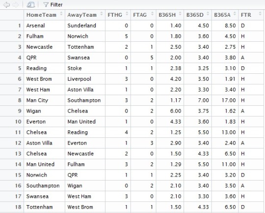
4. Extract following information from dataset

HomeTeam = Home Team
AwayTeam = Away Team
FTHG = Full Time Home Team Goals
FTAG = Full Time Away Team Goals
FTR = Full Time Result (H=Home Win, D=Draw, A=Away Win)
B365H = Bet365 home win odds
B365D = Bet365 draw odds
B365A = Bet365 away win odds

The reason I want to include Bet365 is because I think bets tell a lot about the current performance of the team which the match result doesn't tell. 
5. Combine all 4 files of dataset into one.

file1 <- read.csv("~/My Received Files/2010.csv", header = TRUE, stringsAsFactors = FALSE)
file2 <- read.csv("~/My Received Files/2011.csv", header = TRUE, stringsAsFactors = FALSE)
file3 <- read.csv("~/My Received Files/2012.csv", header = TRUE, stringsAsFactors = FALSE)
file4 <- read.csv("~/My Received Files/2013.csv", header = TRUE, stringsAsFactors = FALSE)
file5 <- read.csv("~/My Received Files/2014.csv", header = TRUE, stringsAsFactors = FALSE)

f1f2 <- rbind(file1, file2)
f4f5 <- rbind(file4, file5)
f1clean <- f1f2[,c(3,4,5,6,24,25,26,7)]
f2clean <- f4f5[,c(3,4,5,6,24,25,26,7)]
f3clean <- file3[,c(3,4,5,6,23,24,25,7)]
f2combine <- rbind(f1clean, f2clean)
finalfile <- rbind(f3clean, f2combine)

Rbind function : Combines  matrix, vactor or dataframe by values.

6. Save the dataframe to CSV file
write.csv(finalfile ,"~/My Received Files/test.csv")
7. Sort in alphabetical order.
teams = sort(unique(c(as.character(finalfile$HomeTeam), as.character(finalfile$AwayTeam))))
8. Create a table to store the wins and point record of each team. For that we create an empty data frame called final table with below columns.

finaltable = data.frame(Team = teams,
                     Games = 0, Win = 0, Draw = 0, Loss = 0, PercentWins=0,
                     HomeGames = 0, HomeWin = 0, HomeDraw = 0, HomeLoss = 0, percentHomeWins =0,
                     AwayGames = 0, AwayWin = 0, AwayDraw = 0, AwayLoss = 0, percentAwayWins =0)

9. Store in the above table count of matches all teams we can use the function as.numeric for that

finaltable$HomeGames = as.numeric(table(finalfile$HomeTeam))
finaltable$AwayGames = as.numeric(table(finalfile$AwayTeam))

10. Fill other columns based on values.
The values can be filled using FTR.  Extract the hometeam column of the dataset and see if the FTR column is H, D or A.  Group all these together first based on FTR H then based on team.  Similarly for D and A. and also for win and loss.

finaltable$HomeWin =
 as.numeric(table(finalfile$HomeTeam[finalfile$FTR == "H"]))
finaltable$HomeDraw =
 as.numeric(table(finalfile$HomeTeam[finalfile$FTR == "D"]))
finaltable$HomeLoss =
 as.numeric(table(finalfile$HomeTeam[finalfile$FTR == "A"]))
finaltable$AwayWin =
 as.numeric(table(finalfile$AwayTeam[finalfile$FTR == "A"]))
finaltable$AwayDraw =
 as.numeric(table(finalfile$AwayTeam[f7$FTR == "D"]))
finaltable$AwayLoss =
 as.numeric(table(finalfile$AwayTeam[f7$FTR == "H"]))

11. Calculate total wins, games,draw  and loss. by adding the total for Home and Away games.

finaltable$Games = finaltable$HomeGames + finaltable$AwayGames
finaltable$Win = finaltable$HomeWin + finaltable$AwayWin
finaltable$Draw = finaltable$HomeDraw + finaltable$AwayDraw
finaltable$Loss = finaltable$HomeLoss + finaltable$AwayLoss

12. Calculate percent wins for total, home and away wins.

finaltable$PercentWins = floor((finaltable$Win / finaltable$Games)*100)
finaltable$percentHomeWins = (finaltable$HomeWin / finaltable$HomeGames)*100
finaltable$percentAwayWins = (finaltable$AwayWin / finaltable$AwayGames)*100

13. Simply graph to extract top 10 teams

finaltable = finaltable[order(-finaltable$PercentWins),]
graphtable = finaltable[1:7,]
graphdata = finaltable[,c(1,5,10,15)]
barplot(graphtable$PercentWins, main="Top Teams in EPL by percent wins", xlab="Teams",
       ylab="PercentWins", names.arg=c("ManCity","United","Chelsea","Arsenal","TTham","Liverpool","Everton"),
       border="blue",col=rainbow(7),fill = rainbow(7))

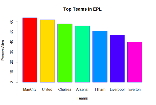
ManCity holds the record of maximum wins in last 5 years, followed closely by Man united and chelsea.

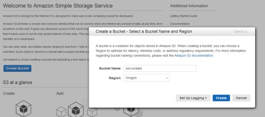
14. Add data to S3.Since AWS ML uses S3 as data storage, you need to upload your data to S3. Create a bucket in S3 and upload the dataset created above to it. This is our test data and all predictions will be based on it. Our dataset is in CSV format as required by AWSML

15. Open AWS  Console : https://console.aws.amazon.com/machinelearning/
Next step is to create a ML model and link the S3 dataset.
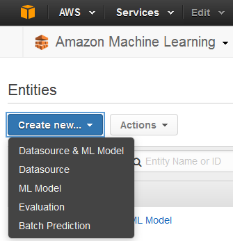
Create new datasource. You can specify data location to be either S3 or redshift.

Spark Streaming

In my previous post I mentioned about Spark Stack. In this post I am to give a brief overview of the component Spark Streaming.

Spark Streaming is an extension to Apache Spark that allows processing of live streams of data.

Data in Spark can be ingested from Kafka, Flume, Twitter or TCP sockets. 

Live Data is broken into chunks/batches for predefined interval of time. Each chunk of data represents an RDD and is processed using RDD operations. Once the operations are performed the results are returned in chunks.

DStream is a basic abstraction in Spark Streaming. They represent a chunk of data and as such implemented as an RDD. Dstreams are created from streaming input sources like Kafka, Twitter etc or by applying transformation operations on existing DStream.

Spark Streaming

The incoming data as mentioned above is processed in predifined interval. All the data for any interval is stored across the cluster for that interval. This results in creation of a dataset. Once the time interval is completed dataset is processed using various operations. The operations could be map-reduce or join. 

Streaming Context is the main entry point of spark application.

val sc = new StreamingContext(sparkContext, seconds(1))

Using sc, Dstreams can be created that represents streaming data from input sources ex. TCP/Twitter. 

TCP

val sData = ssc.socketTextStream("1.2.3.4", 1000)

Here First parameter represents Ip address and second port number. sData represents Dstream of data that will be received from server.

Twitter

val tData = TwitterUtil.createStream(ssc, oauth)

Where oauth denotes the Oauth. Twitter uses Ouath for authorization requests.

Once this is done transformations are applied on the created RDD. One such transormation is flatMap. 

val hashTag = tData.flatMap(status => getTag(status))

val words = sData.flatMap(_.split(" "))

flatMap is an operation that is similar to map but each input is mapped to 0 or more output items resulting in a sequence of data as output. 

Apache Spark a brief overview

Apache Spark a PHD resarch project at UCBerkley came into limelight when it broke the record of sorting petabyte of data recently.
Various Sorting Records.
Databrick



What is Spark ?

Apache Spark™ is a fast cluster computing framework and general engine for large-scale data processing.

Spark Goals:
Generality : Diverse workloads, operators, jobsizes.
Latency:Low Latency
Fault Tolerance


Spark supports Hadoop, Amazon S3, Cassandra, cluster management tools like YARN and Mesos. Spark does more In memory data processing as compared to DiskBased processing as in Hadoop.

Spark stack comes bundled with tools like Spark SQL, MLlib, Spark Streaming and GraphX.

1. SparkSQL: Unified access to structured data , provides compatibility with Apace Hive and Standard Connectivity to tools like JDBC and ODBC.
2. Spark Streaming:  For Scalable fault tolerant Streaming applications and spark can run in both batch and interactive mode.
3. MLlib:Scalable Machine Learning library.
4. GraphX:Large Scale Graph Processing Framework.

Learn More about Spark


Spark vs Hadoop

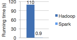
Spark is 100X times faster then Hadoop.
The speed can be attributed to the fact that Spark keeps the intermediate data cached in local JVM.  Hadoop on the other hand in the name of Fault Tolerance write the intermediate data on to the disk and disk is expensive.
                                                                                                               *Image from Spark

Spark doesnt replace anything in Hadoop Ecosystem rather it offers a readable, testable way to write programs freeing us from the painful Map Reduce jobs. MR model is unsuitable for Iterative algorithms. MR jobs are pain to program too. Although there are tools to reduce our efforts in writing MR jobs like Hive, Cascading etc but internally they call MR jobs thus not improving the performance.

Spark programming model
The main abstraction for computation in Spark is Resilient(Can start automatically) Distributed Datasets.

What is RDD ? 
RDD(Spark Paper) :

RDD's are fault-tolerant, parallel data structures that let users explicitly persist intermediate results in memory, control their partitioning to optimize data placement, and manipulate them using a rich set of operators.

Spark transformations applies same data operation to many data items. This results in better Fault tolerance as only the lineage of transformation is logged rather then the actual data. Also if some of RDD's are lost it has enough information to how it is derived from other  RDD's.
RDD can be created through Transformations(map,filter,join). Spark creates Direct Acyclic Graph of these transformation . Once the RDD's are defined through transformations , actions can be applied on them.
Actions are application that returns a value(count,collect and save). In Spark RDD's can be stored in disk by calling persist.
Since it is just an RDD it can be queried via SQL Interface, ML algos etc.

In short
User Program => 
Create Spark Context
sc = new SparkContest
Create Distributed Datasets called RDD's 
Perform Operations.

Inside spark context act as client and master per application.

Block tracker => What is in memory what is on Disk ?
Shuffle => Shuffle operation like Groupby

Scheduler talk through cluster manager talks to a worker.
Contains Block Manager for Block Mgmt.
Recieves task that run in thread pools.
Task can talk to HDFS.

A * Star Algorithm

A* is a path finding/Graph Traversal  algorithm generally used in game programming to determine the shortest path to reach a particular destination following Best First Search approach. Can be called as an extension of Dijkstra and reduces the number of comparisons while guaranteeing optimality. Heuristic is used in A*. A* uses heuristic to determine most promising node.   

Consider a grid with each square numbered. As in the above figure , cross sign (Sq. 14) represents start point and cross sign (Sq 35) represents destination. All Blue bars in a square represents the block. 
Each square considered a node.
Some terminology used with A*
Node Data
H Value :  Heuristic Value
G Value : Movement Cost                
F Value : G + H Value
Parent :  Pointer Back to previous node.

List
Open Node : List of Nodes to be visited
Close Node :  Already Visited.

Task : Shortest Path from 14 to 35.
H Value : Distance of a Node from destination node in our case from Sq 35.
Precompute all H value

If H value is Zero A* behaves like Dijksatra Algorithm. From Node 17 H value is 3 as you can go from 17 to 23 to 29 leading to 35
For Node 25 H value is 5 as you go from node 25 to 26 to 27 to 28 to 29 leading to 35 , block nodes are also considered for precomputing H values.

G Value is movement cost from Start node to another node.
Consider Movement cost of 10 For Horizontal and Vertical and of 14 for diagonal movement.
Diagonal > Horizontal (Pythagorean theoram)
So to Move from 14 to 8 the cost is 10 and from 14 to 9 it is 14.
Each square has parents.
For Sq. 14 we need to get parent , which can be done through open list and close list.
Write now no node on Close or open list.

All Node parent to14.
CloseList : 14
Open List : 7,8,9,13,15,19,20,21
Calculate G Cost for all. for 8 it is for Node 14 it is 0 for Node 8 it is 10 so total is 5. For Node 9 it is 14.

The Numbers in Black represents the H value of Nodes ie Distance of Node to Node 35.
The numbers in Blue represent G Value Node 8 as G Value 10.
F Value is sum of G Value + H Value which is written in red for the nodes. (For node 7 it is 17 => 10+7)
Need to Use Node with smallest F Value.
So in our case square number 15 as it has F-Value 15 which is minimum. Node 20 too has value 15 and can be selected too.
Take Node 15 put in close list.
Now repeat process for Node 15.

Now Calculate all values for Node 15.
CloseList : 14 , 15
Open List : 7,8,9,13,19,20,21,10
We see Node 14 already on Close list dont do anything.
Consider Node 8 so we check if it is more faster to go to 8 from 14 or  from 15.
For Node 15 We see :
G Value for Node 15 was 10 . G Value for Node 8 considering the current node 14 is 14
So total Movement is 14+10 ie 24
If the total movement > current G value dont change values else
If G value wrt node 15 is less then G Value of Node 8 then re parent node  8 to node 15.

If(Parents G value+Current G < Parents New G){
Add new Block to close list.
New Block parent = Prev Block Parent.
}


This process continues till you are next to destination node.

Closed : 14,15,20
Open : 7,8,9,13,19,21,10,22,25,27
Keep Doing and then see neighbor is destination so make destination parented to the other node and you are done.
Trace back path from destination to source.
35 to 29 to 22 to 15 to 14.
Make sure you change the parent if you find new G value smaller then previous computed.

All Green Arrow denotes final position of main node parents. Red is the path from source to destination.

Shortest Path : 14 ->15->22->29->35

   

 
Useful links for the topic 

Wiki
Stanford Amits Page
Video  
Video
Video
Algo
 

Understanding Evaluation Metrices.

Confusion Matrix is a tabular layout that can be used to measure the performance of an algorithm. Each Column represents predicted value and each row represents actual value. 
Lets take an example of testing a person for cancer. 
If the person has cancer , the test will say it as positive and if not then negative.
There are can be 4 outcomes if we consider test as an experiment.

1) The patients were suffering from cancer and our test recognized them as suffering from Cancer : These are called TRUE POSITIVE.
2) The patients were suffering from cancer but tests showed negative : These are called TRUE NEGATIVE
3) Patients who were healthy but were diagnosed as suffering from Cancer : FALSE POSITIVE
4) Patients who were not suffering from cancer and test said the same : FALSE NEGATIVE.

Precision (Positive Predicted Value) : proportion of patients test showed as having cancer and they actually had cancer.

  
Recall(True Positive Rate)  : proportion of patients that actually had Cancer were diagnosed by test as having cancer. :

 
Precision and Recall Inversely Related

Accuracy : 
Ratio of Correctly classified instances to total instances.
In layman terms : Number of times the test were right 

Where P and N are total number of tests.


F1 :  is a measure that combines the precision and recall rates by computing the harmonic mean between them. F-Measure does not consider True Negatives into account. 

ROC Curve
Receiver Operating Curve(ROC)  is a plot to show change in performance of Binary Classifier with change in Threshold. The graphs are plotted as the fraction of true positive by total actual positive called the TRUE POSITIVE RATE and true negatives by total actual negatives also called the TRUE NEGATIVE RATE. Values range between 0 and 1.

 

Python and NLP

I recently worked on a project titled "Recommending Similar defects on Apache Hadoop" .Its a recommendation system that predicts similar defects and then predicts the effort estimate for each defect.

Steps:

1) Extract XML/Excel data from Apache Hadoop Issue Tracker.

https://issues.apache.org/jira/browse/HADOOP

2)Convert the extracted data into CSV for persistent storage.

3)Extract required Column

Python COde :

import csv
import re

def col_selector(table, column_key):
    return [row[column_key] for row in table]

with open("Data/next.csv","r") as csvfile:
    reader = csv.DictReader(csvfile, delimiter=",")
    table = [row for row in reader]
    foo_col = col_selector(table, "Summary")
    bar_col = col_selector(table, "Description")

The above example extract two columns from Apache Hadoop Issue Tracker CSV file.  Your program must include python library called csv.py

http://docs.python.org/2/library/csv.html

4)From these Column we will generate a set of words specific to Hadoop.

We will apply various NLP to generate various words from the summary and description.

5)There are 5 Steps in Natural Language Processing 

1. Tokenizing
2. Stemming
3. Stop Word Removal
4. Vector Space Representation
5. Similarity Measures

Step 1 : Tokenizing :

 The tokenization process involves breaking a stream of characters of text up into words or phrases, symbols or other meaningful elements called tokens. Before indexing, we Fillter out all common English stopwords.I obtained a list of around 800 stopwords online. 

K. Bounge. Stop Word List.
https://sites.google.com/site/kevinbouge/stopwords-lists

The list contained articles, pronouns, verbs etc. I filtered out all those words from our extracted text. After reviewing the list, we felt stopwords list for a Hadoop Database has to be built separately, as numbers and sym-
bols are also to be filtered out. 

Step 2:
Stemming is used to try to identify a ground form for each word in the text. Some words that carry the same information can be used in different grammatical ways, depending on how the creator of the report wrote it down. This phase will remove a xes and other components from each token
that resulted from tokenization so that only the stem of each word remains. For stemming, we used a python library called PortorStemmer. We passed to it stream of extracted words. Words like caller, called, calling whose stem was call were Filtered and only 1 word, call, was kept in the nal list.I Filtered around 1200 words this way.

Step 3:
Stop Word Removal 
Synonyms removal and replace by 1 common word.I used wordnet NLTK to perform this.
Second Phase : Spell checking: List compared with list of misspelled words.

Step 4:
Vector Space representation.
After the first 3 steps I had around 5500 words. These words were used to identify tags.Each defect with tags was then represented into a Vector space model.Used general method used by scikit.

Step 4: Similarity Measure.
Calculated the cosine similarity between the two defect vectors.
 

Supervised Learning : A Mathematical Foundation

Supervised Learning as per Wiki

Supervised learning is the machine learning task of inferring a function from labeled training data. The training data consist of a set of training examples. In supervised learning, each example is a pair consisting of an input object (typically a vector) and a desired output value (also called the supervisory signal). A supervised learning algorithm analyzes the training data and produces an inferred function, which can be used for mapping new examples. An optimal scenario will allow for the algorithm to correctly determine the class labels for unseen instances.

In Short : Learning from historical data a mapping between input and output variables and applying this to predict output for an unseen data.

STEPS of SUPERVISED LEARNING

• Determine type of training example

• What kind of data to be used.

• Handwriting analysis : single handwritten character, word,line

• Gather a Training set

• Determine Input feature representation of learned function.

• Input object transformed into feature vector.

• Determine structure of learned function and corresponding learning algorithm.

• SVM or DT

• Complete the design.

• Run Algorithm on Training set.

• Evaluate accuracy.

 Mathematics behind Supervised Learning

Goal : Infer a function

f : X → Y

Classifier from sample data A_n

_{An = ((x1, y1), ..., (xn, yn)) ∈ (X × Y )ⁿ.}

_{Input and Output points} x_i and y_i ∈ Y 

y_i ∈ IR for regression problems, and y_i is discrete for classification problems {-1, +1}

 

_{2 Hypothesis :} 

_{1)Find a function f to model depandency in P(x,y)} 

_{2)Error or loss between prediction f(x) desired output y.}  

_{Loss function :} L : Y ×Y → IR⁺

If Binary Classification Y in {-1,+1}   L( h (x), y)) = ^1/₂ | h(x) − y|.

Unsupervised Learning a function can be

L_u( h(x)) = −log( h(x)).

 Risk for a function or Generalization Error 

R( h ) =    L( h(x), y)dP(x, y). 

Classification : Function f that minimises R(f) but joint probablity P(x,y) unknown

 Using Input and Random variables Risk can be written as 

Empirical Risk Minimisation : 

Learning algo find Hypothesis h such that R(h) minimum

R(h) cannot be computed  so approximation Empirical Risk by leveraging loss  

for Large numbers As m goes to infinity point wise convergence of h to R(h)

Minimise Rem

 

 

Consistency is important : 

 

Thus learning depands upon function h or f in above case 

It has to have smooth boundries , regularization is applied : Regularization theory.

Regularized Risk : 

Ω ( f ) : Roughness Penalty

Risk Bounds 

H , A_n and δ , such that, for any f ∈ H , with a probability at least 1 − δ :

 

consider the case of a finite class of functions, |H | = N.   

Hoeffding Inequality by summing over set : 

  Risk =  sum of 2 terms : Empirical error and bound depand on size.

 As n -> infintiy second term tends to 0

Bias Variance Dilemma

H large one can find f that fits the data but noise due to large points resulting in poor performance 

Called Overfitting 

Overfitting according to Wiki

Generally, a learning algorithm is said to overfit relative to a simpler one if it is more accurate in fitting known data (hindsight) but less accurate in predicting new data (foresight).

VC dimension

Measure of capacity of function to different label of class

 

 

STRUCTURAL RISK MINIMISATION

Structural risk minimization seeks to prevent overfitting by incorporating a regularization penalty into the optimization. The regularization penalty can be viewed as implementing a form of Occam's razor that prefers simpler functions over more complex ones

 

 

select classifier that maximizes gamma  .



*Formulas taken from paper by cunningham  
http://tinyurl.com/ll4jxhq