Data Analytics with Amazon Machine Learning - Premier League Data

Dataset Source : Soccer 
Use Case and Dataset
The most important part of any machine learning application is to get the right dataset. As I am very much interested in Soccer, I thought of using the previous Premier league to predict winner of this season.
I agree that winner prediction is arguable and its hard to predict the winners due to so many factors associated, but I just want to try my hands on the new machine learning framework released by amazon few days back called “AWS Machine Learning ”.  
Steps :
1. Download last 5 years of Premier League data from the website (2010-2015).
2. Data From (2010-2014)  will be the training data.
3. 2015 will be the test data.
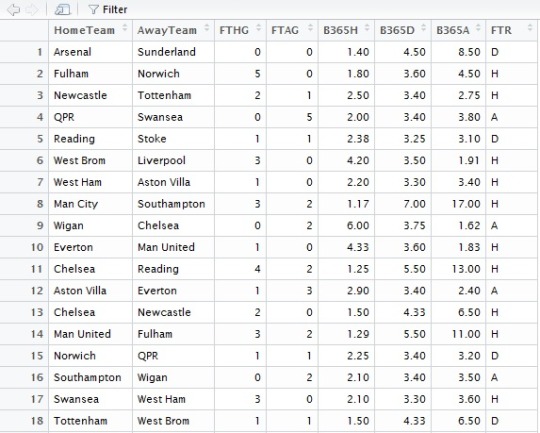
4. Extract following information from dataset

HomeTeam = Home Team
AwayTeam = Away Team
FTHG = Full Time Home Team Goals
FTAG = Full Time Away Team Goals
FTR = Full Time Result (H=Home Win, D=Draw, A=Away Win)
B365H = Bet365 home win odds
B365D = Bet365 draw odds
B365A = Bet365 away win odds

The reason I want to include Bet365 is because I think bets tell a lot about the current performance of the team which the match result doesn't tell. 
5. Combine all 4 files of dataset into one.

file1 <- read.csv("~/My Received Files/2010.csv", header = TRUE, stringsAsFactors = FALSE)
file2 <- read.csv("~/My Received Files/2011.csv", header = TRUE, stringsAsFactors = FALSE)
file3 <- read.csv("~/My Received Files/2012.csv", header = TRUE, stringsAsFactors = FALSE)
file4 <- read.csv("~/My Received Files/2013.csv", header = TRUE, stringsAsFactors = FALSE)
file5 <- read.csv("~/My Received Files/2014.csv", header = TRUE, stringsAsFactors = FALSE)

f1f2 <- rbind(file1, file2)
f4f5 <- rbind(file4, file5)
f1clean <- f1f2[,c(3,4,5,6,24,25,26,7)]
f2clean <- f4f5[,c(3,4,5,6,24,25,26,7)]
f3clean <- file3[,c(3,4,5,6,23,24,25,7)]
f2combine <- rbind(f1clean, f2clean)
finalfile <- rbind(f3clean, f2combine)

Rbind function : Combines  matrix, vactor or dataframe by values.

6. Save the dataframe to CSV file
write.csv(finalfile ,"~/My Received Files/test.csv")
7. Sort in alphabetical order.
teams = sort(unique(c(as.character(finalfile$HomeTeam), as.character(finalfile$AwayTeam))))
8. Create a table to store the wins and point record of each team. For that we create an empty data frame called final table with below columns.

finaltable = data.frame(Team = teams,
                     Games = 0, Win = 0, Draw = 0, Loss = 0, PercentWins=0,
                     HomeGames = 0, HomeWin = 0, HomeDraw = 0, HomeLoss = 0, percentHomeWins =0,
                     AwayGames = 0, AwayWin = 0, AwayDraw = 0, AwayLoss = 0, percentAwayWins =0)

9. Store in the above table count of matches all teams we can use the function as.numeric for that

finaltable$HomeGames = as.numeric(table(finalfile$HomeTeam))
finaltable$AwayGames = as.numeric(table(finalfile$AwayTeam))

10. Fill other columns based on values.
The values can be filled using FTR.  Extract the hometeam column of the dataset and see if the FTR column is H, D or A.  Group all these together first based on FTR H then based on team.  Similarly for D and A. and also for win and loss.

finaltable$HomeWin =
 as.numeric(table(finalfile$HomeTeam[finalfile$FTR == "H"]))
finaltable$HomeDraw =
 as.numeric(table(finalfile$HomeTeam[finalfile$FTR == "D"]))
finaltable$HomeLoss =
 as.numeric(table(finalfile$HomeTeam[finalfile$FTR == "A"]))
finaltable$AwayWin =
 as.numeric(table(finalfile$AwayTeam[finalfile$FTR == "A"]))
finaltable$AwayDraw =
 as.numeric(table(finalfile$AwayTeam[f7$FTR == "D"]))
finaltable$AwayLoss =
 as.numeric(table(finalfile$AwayTeam[f7$FTR == "H"]))

11. Calculate total wins, games,draw  and loss. by adding the total for Home and Away games.

finaltable$Games = finaltable$HomeGames + finaltable$AwayGames
finaltable$Win = finaltable$HomeWin + finaltable$AwayWin
finaltable$Draw = finaltable$HomeDraw + finaltable$AwayDraw
finaltable$Loss = finaltable$HomeLoss + finaltable$AwayLoss

12. Calculate percent wins for total, home and away wins.

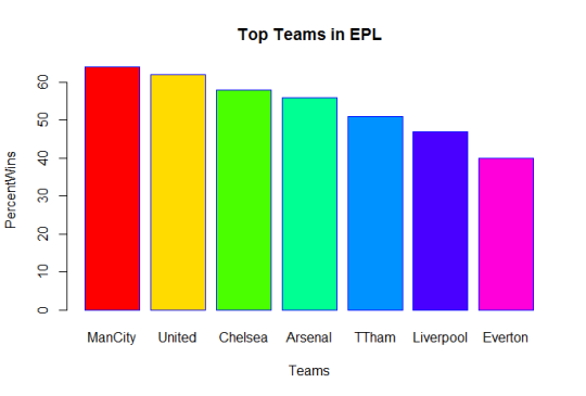
finaltable$PercentWins = floor((finaltable$Win / finaltable$Games)*100)
finaltable$percentHomeWins = (finaltable$HomeWin / finaltable$HomeGames)*100
finaltable$percentAwayWins = (finaltable$AwayWin / finaltable$AwayGames)*100

13. Simply graph to extract top 10 teams

finaltable = finaltable[order(-finaltable$PercentWins),]
graphtable = finaltable[1:7,]
graphdata = finaltable[,c(1,5,10,15)]
barplot(graphtable$PercentWins, main="Top Teams in EPL by percent wins", xlab="Teams",
       ylab="PercentWins", names.arg=c("ManCity","United","Chelsea","Arsenal","TTham","Liverpool","Everton"),
       border="blue",col=rainbow(7),fill = rainbow(7))

ManCity holds the record of maximum wins in last 5 years, followed closely by Man united and chelsea.

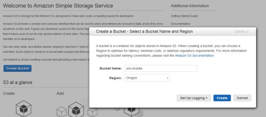
14. Add data to S3.Since AWS ML uses S3 as data storage, you need to upload your data to S3. Create a bucket in S3 and upload the dataset created above to it. This is our test data and all predictions will be based on it. Our dataset is in CSV format as required by AWSML

15. Open AWS  Console : https://console.aws.amazon.com/machinelearning/
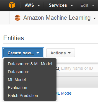
Next step is to create a ML model and link the S3 dataset.
Create new datasource. You can specify data location to be either S3 or redshift.

Data Analytics with R - World Bank Refugee Population data

Data Source :  World Bank Data
Problem :  To observe the distribution of refugees across the globe in past two decades.

Data Cleaning : Removed all countries with <100 people as refugees. Remove all unnecessary columns with no relevent data like Indicator name, Indicator code.
Step 1: 
1. Install R
2. IDE : RSTudio,
3. Online Editor : Data Joy.
4. Loading dataset in R:

df <- read.csv("data.csv", stringsAsFactors=FALSE)

this create an object by name mydf. Each cell in a CSV file is in a delimiter seperated format, mostly the delimiter is comma but there can be others as well.  The first row contains the header in this case “Country Name “, “Country Code” and the refugee population between years 1990-2013. We can prevent conversion of string to factor( A type) in R by setting stringAsFactors to false. By default it is true.

5. To check all the column names :
In the console type : 

• str(df)This function compactly displays the Structure of an R Object.  All the column headers with data type wil be displayed.

2 char columns are Country Name and Code. The rest are number of people that seek refugee in the specific country.

6. To access columns of a dataframe,
You can use :

table(mydf$Country.Name)

To get header names use :

print(names(df))

Table command will return you a vector with value in column Country.Name and the count of that value, since these values are population of refugees, which is unique it gives you count 1.

Afghanistan                  Albania                  Algeria                                               1                                        1                          1

To get the proportion one can use :

prop.table(table(mydf$Country.Name))

Though not required for this data.
7.  Create a new column Category in the data frame

df$Category  <- mydf$Country.Code

8. To get the upper limit of our data, we need to get the maximum number of refugees by a country in particular column. For Year 2013 the maximum value can be extracted using:

max(df$X2013, na.rm = TRUE)

9. There are some countries in dataset where the columns are either not available or empty, resulting in a lot of “NA” in the data. Lets convert all Empty columns to a numerical value of 1(~0).

df[is.na(df)] <- 1

In ‘R’ the value is assigned using ‘<-‘ operator, this makes all ‘NA’ columns as 1.

10.  Since the dataset has  highly varying range of values, ranging from 1 to 2712888, I decide to categories them into different categories. The idea is to create a bucket distirbution. Each bucket will have some capacity, in this case say 10000.  

Bucket 1 : 1- 9999 (All entries between 1-9999 will be in this bucket.
Bucket 2:  10000-19999
and so on.

11. Now we have to loop through every cell value in the data frame and replace it with the bucket they fall into.

for(i in names(df)){if((i != colnames(df)[1]) && (i != colnames(df)[2]) && (i != colnames(df)[18])){

      sq<-seq(0,3000000,10000)
      qr<- cut(df[,i],sq,labels = c(1:300))
      df[,i]<-as.numeric(qr)
   }
}

Excluding all values in the first (Country Name column), second (Country Code column), last column which we created previously called Category.
R provides a method called cut: cut converts the range of values into intervals and assigns the values in x according to which interval they fall.

cut((x, breaks, labels = NULL, ...))
X : a numeric vector which is to be converted to a factor by cutting.
breaks : breaks either a numeric vector of two or more unique cut points
labels”  labels for the levels of the resulting category.

A intermediate factor vector is created for each column and the resulting value of the column is updated with it.  SInce this is a factor vector, the value is typecast to numeric in the next line. If the number of cut points doesn't match based on the cut, an error will be thrown “Length do not match”

No of cutpoint = Data Max Value / Capacity of bucket

12. Convert your data to long format as needed by ggplot
GGPlot is a graph plotting library of R.
Reshape2 is a transformation library.

Library(reshape2)
df.molten <- melt(df, value.name="Count", variable.name="Year", na.rm=TRUE)

13. Plot the graph using ggplot’s qplot by categories.

par( mfrow = c(3,3) )

library(ggplot2)

qplot( data=df.molten, x = Year,y = Count, geom="bar", size = I(2),stat = "identity" ,las=0.3, cex.names=0.4) + facet_wrap( "Category" ) + geom_bar(width=1.5)

14. Some useful information retrieved from data :
a ) Number of refugees increasing every year.
b) Huge rise in number of refugees in European countries in last few years
c) Jordon, Pakistan, Iran and Germany has most number of refugees.
d) Sweden refugees are increasing at an alarming pace, but lesser then last few years.
e) Most of the countries are very much constant with the number of refugees they allow in their home country esp Chech Republic, Greece, India, and China,
f) In European countries Germany (Country Code - DEU) has the highest number of refugees.
g) There is a large uneven distribution of refugees across europe, some countries <1000 refugees and some numbers are too high.
h) United States also has a large number of refugee population and it is just second to Germany(excluding middle eastern states) in terms of numbers.
i) There has been sudden rise in number of refugees especially in Gaza, Syria, Canada, Britain.
f) Iran, Zimbabwe, Saudi Arabia Ghana has seen big decline in past few years .
g) The number if refugees in Saudi Arabia, UAE, Russia and Qatar are alarmingly low.
h) Number of refugees in Europe is rising. Germany, France, United Kingdom and Sweden and Turkey leads in number of refugees.

Playing with Tumblr API

1. Install Ouath2
2. Install Pytumblr
3. Register an Application
https://www.tumblr.com/oauth/apps
4. Get tumblr ouath2, you will get once you create app
5. Enter your credentials in following code in Python file

client = pytumblr.TumblrRestClient(
    '<consumer_key>',
    '<consumer_secret>',
    '<oauth_token>',
    '<oauth_secret>',
)

pytumblr is a library,  through which you can make calls to tumblr.

6. Code to get all blogs you are following

off =0
while True:
    my_dict = client.following(offset =off)
    res = my_dict['blogs']
    for rs in res:
        print(rs['name'] + "...." + rs['title'])
   
       
    off+=20

7. Number of posts liked for each blog

off =0
like_dict= {}
while True:
    my_dict = client.blog_likes('conflatedthought.tumblr.com',offset =off)
    res = my_dict['liked_posts']
    for rs in res:
        strs = str(rs['tags']).strip('[]')
        #print(rs['blog_name'] +" "+ strs)
        #print("..")
        if rs['blog_name'] in like_dict.keys():
            like_dict[rs['blog_name']] += 1
            #print rs['blog_name'] +"  " + str(like_dict[rs['blog_name']])
        else:
            like_dict[rs['blog_name']] = 1   
          
    off+=20
for the_key, the_value in like_dict.iteritems():
    print the_key, 'corresponds to', the_value 

8. Sample Output for code 6

sportspage....Sports Page
themobilemovement....The Mobile Movement
adidasfootball....adidas Football
instagram-engineering....Instagram Engineering
soccerdotcom....SOCCER.COM
sony....Sony on Tumblr
yahoolabs....Yahoo Labs
taylorswift....Taylor Swift
beyonce....Beyoncé | I Am
itscalledfutbol....Did someone say "futbol"?
futbolarte....Futbol Arte
fcyahoo....FC Yahoo
yahooscreen....Yahoo Screen
yahoo....Yahoo
engineering....Tumblr Engineering
yahoodevelopers....Yahoo Developer Network
mongodb....The MongoDB Community Blog
yahooeng....Yahoo Engineering
marissamayr....Marissa's Tumblr
staff....Tumblr Staff
whoagurt....Whoagurt
narendra-modi....Narendra Modi
nytvideo....New York Times Video
bonjovi-is-my-life....Bon Jovi♥ Is My Life
etsy....Etsy
game-of-thrones....You win or you die.
seinfeld....Seinfeld
itunes....iTunes
teamindiacricket....Team India
gameofthrones....Game of Thrones: Cast A Large Shadow
forzaibra....Forza Ibra

Tumblr Blog

My Tumblr Blog
 

 
Why I am moving to tumblr :
1. Lots of stuff to read
2. Simple to use.
3. 230 Million Blogs
4. No Charge.
5. Great Design optimized for Mobile.
6. Easier to get followers


7. I am joining Yahoo :)

My blog will remain active but most of the new post will be on tumblr.

Spark Streaming

In my previous post I mentioned about Spark Stack. In this post I am to give a brief overview of the component Spark Streaming.

Spark Streaming is an extension to Apache Spark that allows processing of live streams of data.

Data in Spark can be ingested from Kafka, Flume, Twitter or TCP sockets. 

Live Data is broken into chunks/batches for predefined interval of time. Each chunk of data represents an RDD and is processed using RDD operations. Once the operations are performed the results are returned in chunks.

DStream is a basic abstraction in Spark Streaming. They represent a chunk of data and as such implemented as an RDD. Dstreams are created from streaming input sources like Kafka, Twitter etc or by applying transformation operations on existing DStream.

Spark Streaming

The incoming data as mentioned above is processed in predifined interval. All the data for any interval is stored across the cluster for that interval. This results in creation of a dataset. Once the time interval is completed dataset is processed using various operations. The operations could be map-reduce or join. 

Streaming Context is the main entry point of spark application.

val sc = new StreamingContext(sparkContext, seconds(1))

Using sc, Dstreams can be created that represents streaming data from input sources ex. TCP/Twitter. 

TCP

val sData = ssc.socketTextStream("1.2.3.4", 1000)

Here First parameter represents Ip address and second port number. sData represents Dstream of data that will be received from server.

Twitter

val tData = TwitterUtil.createStream(ssc, oauth)

Where oauth denotes the Oauth. Twitter uses Ouath for authorization requests.

Once this is done transformations are applied on the created RDD. One such transormation is flatMap. 

val hashTag = tData.flatMap(status => getTag(status))

val words = sData.flatMap(_.split(" "))

flatMap is an operation that is similar to map but each input is mapped to 0 or more output items resulting in a sequence of data as output.